The R package fable.binary provides a collection of time series forecasting models suitable for binary time series. These models work within the fable framework, which provides the tools to evaluate, visualise, and combine models in a workflow consistent with the tidyverse.
Installation
You can install the development version from GitHub
# install.packages("remotes")
remotes::install_github("tidyverts/fable.binary")
Examples
library(fable.binary)
#> Loading required package: fabletools
library(ggplot2)
library(dplyr)
#>
#> Attaching package: 'dplyr'
#> The following objects are masked from 'package:stats':
#>
#> filter, lag
#> The following objects are masked from 'package:base':
#>
#> intersect, setdiff, setequal, union
# Fit models
fit <- melb_rain |>
model(
nn = BINNET(Wet ~ fourier(K = 1, period = "year")),
logistic = LOGISTIC(Wet ~ fourier(K = 5, period = "year"))
)
# Functions for computing on models
fit |> tidy()
#> # A tibble: 11 × 6
#> .model term estimate std.error statistic p.value
#> <chr> <chr> <dbl> <dbl> <dbl> <dbl>
#> 1 logistic "(Intercept)" -0.573 0.0321 -17.8 3.18e-71
#> 2 logistic "fourier(K = 5, period = \"ye… -0.325 0.0458 -7.10 1.26e-12
#> 3 logistic "fourier(K = 5, period = \"ye… -0.279 0.0451 -6.18 6.25e-10
#> 4 logistic "fourier(K = 5, period = \"ye… -0.0203 0.0455 -0.446 6.56e- 1
#> 5 logistic "fourier(K = 5, period = \"ye… -0.0312 0.0453 -0.688 4.91e- 1
#> 6 logistic "fourier(K = 5, period = \"ye… -0.0696 0.0454 -1.53 1.26e- 1
#> 7 logistic "fourier(K = 5, period = \"ye… -0.0207 0.0454 -0.457 6.48e- 1
#> 8 logistic "fourier(K = 5, period = \"ye… -0.0342 0.0454 -0.754 4.51e- 1
#> 9 logistic "fourier(K = 5, period = \"ye… 0.0224 0.0454 0.494 6.21e- 1
#> 10 logistic "fourier(K = 5, period = \"ye… -0.0188 0.0453 -0.415 6.78e- 1
#> 11 logistic "fourier(K = 5, period = \"ye… 0.00815 0.0453 0.180 8.57e- 1
fit |> select(logistic) |> glance()
#> # A tibble: 1 × 12
#> .model df log_lik AIC AICc BIC deviance df.residual rank
#> <chr> <int> <dbl> <dbl> <dbl> <dbl> <dbl> <int> <int>
#> 1 logistic 11 -2787. 5596. 5596. 5666. 5574. 4311 11
#> # ℹ 3 more variables: null_deviance <dbl>, df_null <int>, nobs <int>
fit |> select(logistic) |> report()
#> Series: Wet
#> Model: LOGISTIC
#>
#> Coefficients:
#> Estimate Std. Error t value Pr(>|t|)
#> (Intercept) -0.573059 0.032114 -17.845 < 2e-16 ***
#> fourier(K = 5, period = "year")C1_365 -0.324774 0.045754 -7.098 1.26e-12 ***
#> fourier(K = 5, period = "year")S1_365 -0.278737 0.045075 -6.184 6.25e-10 ***
#> fourier(K = 5, period = "year")C2_365 -0.020283 0.045519 -0.446 0.656
#> fourier(K = 5, period = "year")S2_365 -0.031195 0.045310 -0.688 0.491
#> fourier(K = 5, period = "year")C3_365 -0.069556 0.045449 -1.530 0.126
#> fourier(K = 5, period = "year")S3_365 -0.020730 0.045374 -0.457 0.648
#> fourier(K = 5, period = "year")C4_365 -0.034241 0.045438 -0.754 0.451
#> fourier(K = 5, period = "year")S4_365 0.022435 0.045375 0.494 0.621
#> fourier(K = 5, period = "year")C5_365 -0.018772 0.045275 -0.415 0.678
#> fourier(K = 5, period = "year")S5_365 0.008153 0.045337 0.180 0.857
#> ---
#> Signif. codes: 0 '***' 0.001 '**' 0.01 '*' 0.05 '.' 0.1 ' ' 1
#>
#> # A tibble: 1 × 11
#> df log_lik AIC AICc BIC deviance df.residual rank null_deviance
#> <int> <dbl> <dbl> <dbl> <dbl> <dbl> <int> <int> <dbl>
#> 1 11 -2787. 5596. 5596. 5666. 5574. 4311 11 5668.
#> # ℹ 2 more variables: df_null <int>, nobs <int>
fit |> select(nn) |> glance()
#> # A tibble: 1 × 6
#> .model inputs hidden_nodes weights repeats sigma2
#> <chr> <dbl> <dbl> <int> <int> <dbl>
#> 1 nn 2 2 9 20 0.227
fit |> select(nn) |> report()
#> Series: Wet
#> Model: BINNET: 2
#>
#> Average of 20 networks, each of which is
#> a 2-2-1 network with 9 weights
#> options were -
#>
#> sigma^2 estimated as 0.2269
augment(fit)
#> # A tsibble: 8,644 x 6 [1D]
#> # Key: .model [2]
#> .model Date Wet .fitted .resid .innov
#> <chr> <date> <lgl> <dbl> <dbl> <dbl>
#> 1 nn 2000-01-01 TRUE 0.255 0.745 0.745
#> 2 nn 2000-01-02 FALSE 0.254 -0.254 -0.254
#> 3 nn 2000-01-03 FALSE 0.253 -0.253 -0.253
#> 4 nn 2000-01-04 TRUE 0.252 0.748 0.748
#> 5 nn 2000-01-05 TRUE 0.251 0.749 0.749
#> 6 nn 2000-01-06 FALSE 0.250 -0.250 -0.250
#> 7 nn 2000-01-07 FALSE 0.249 -0.249 -0.249
#> 8 nn 2000-01-08 FALSE 0.248 -0.248 -0.248
#> 9 nn 2000-01-09 FALSE 0.248 -0.248 -0.248
#> 10 nn 2000-01-10 TRUE 0.247 0.753 0.753
#> # ℹ 8,634 more rows
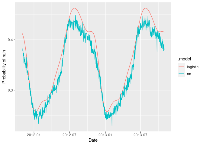
# Produce forecasts. For neural network, use
fc <- forecast(fit, h = "2 years")
as_tibble(fc) |>
ggplot(aes(x = Date, y = .mean, col = .model)) +
geom_line() +
labs(y = "Probability of rain")