4 Accessing model elements
4.1 Display
The print and summary methods are standard displays for fitted models. The print method typically displays a limited amount of key information, such as the model that was fit, and the estimated coefficients. The summary function extends the print method with a more detailed summary of fit, which may include measures for goodness of fit, and significance of model terms.
As fable naturally supports batch/multiple forecasting, the print method is standardised for any number of models. A very short model specific display can be defined using the model_sum generic, which is shown in the mable.
library(tsibbledata)
UKLungDeaths <- as_tsibble(cbind(mdeaths, fdeaths), gather = FALSE)
## Warning: Argument `gather` is deprecated, please use `pivot_longer`
## instead.ets_fit <- UKLungDeaths %>%
model(ETS(mdeaths))## # A mable: 1 x 1
## `ETS(mdeaths)`
## <model>
## 1 <ETS(M,A,A)>The summary method can then be used to reveal more information about this model, such as fitted parameters and goodness of fit. Ideally this information would also be standardised into a tabular form for batch modelling, although this is currently not the case.
ets_fit %>%
  summary
## Length Class Mode
## par 2 tbl_df list
## est 4 tbl_ts list
## fit 8 tbl_df list
## states 15 tbl_ts list
## spec 5 tbl_df list4.2 Fitted values and residuals
Accessors for fitted values and residuals return a tsibble containing the index from the original data, with a measured variables for .fitted values and .resids. If the mable contains more than one model, the resulting object maintains and respects the key structure.
ets_fit %>%
  fitted
## # A tsibble: 72 x 3 [1M]
## # Key: .model [1]
## .model index .fitted
## <chr> <mth> <dbl>
## 1 ETS(mdeaths) 1974 Jan 2278.
## 2 ETS(mdeaths) 1974 Feb 2283.
## 3 ETS(mdeaths) 1974 Mar 2142.
## 4 ETS(mdeaths) 1974 Apr 1776.
## 5 ETS(mdeaths) 1974 May 1442.
## 6 ETS(mdeaths) 1974 Jun 1341.
## 7 ETS(mdeaths) 1974 Jul 1270.
## 8 ETS(mdeaths) 1974 Aug 1160.
## 9 ETS(mdeaths) 1974 Sep 1147.
## 10 ETS(mdeaths) 1974 Oct 1381.
## # … with 62 more rowsets_fit %>%
residuals## # A tsibble: 72 x 3 [1M]
## # Key: .model [1]
## .model index .resid
## <chr> <mth> <dbl>
## 1 ETS(mdeaths) 1974 Jan -0.0633
## 2 ETS(mdeaths) 1974 Feb -0.184
## 3 ETS(mdeaths) 1974 Mar -0.124
## 4 ETS(mdeaths) 1974 Apr 0.0569
## 5 ETS(mdeaths) 1974 May 0.0346
## 6 ETS(mdeaths) 1974 Jun -0.0689
## 7 ETS(mdeaths) 1974 Jul 0.00764
## 8 ETS(mdeaths) 1974 Aug -0.0248
## 9 ETS(mdeaths) 1974 Sep 0.0544
## 10 ETS(mdeaths) 1974 Oct 0.0805
## # … with 62 more rows4.3 Broom functionality
Common features from a model can also be accessed using verbs from the broom package. Again, key structures that exist within the mable are respected.
ets_fit %>%
  augment
## # A tsibble: 72 x 5 [1M]
## # Key: .model [1]
## .model index mdeaths .fitted .resid
## <chr> <mth> <dbl> <dbl> <dbl>
## 1 ETS(mdeaths) 1974 Jan 2134 2278. -0.0633
## 2 ETS(mdeaths) 1974 Feb 1863 2283. -0.184
## 3 ETS(mdeaths) 1974 Mar 1877 2142. -0.124
## 4 ETS(mdeaths) 1974 Apr 1877 1776. 0.0569
## 5 ETS(mdeaths) 1974 May 1492 1442. 0.0346
## 6 ETS(mdeaths) 1974 Jun 1249 1341. -0.0689
## 7 ETS(mdeaths) 1974 Jul 1280 1270. 0.00764
## 8 ETS(mdeaths) 1974 Aug 1131 1160. -0.0248
## 9 ETS(mdeaths) 1974 Sep 1209 1147. 0.0544
## 10 ETS(mdeaths) 1974 Oct 1492 1381. 0.0805
## # … with 62 more rowsets_fit %>%
tidyets_fit %>%
glance## # A tibble: 1 x 9
## .model sigma2 logLik AIC AICc BIC MSE AMSE MAE
## <chr> <dbl> <dbl> <dbl> <dbl> <dbl> <dbl> <dbl> <dbl>
## 1 ETS(mdeaths) 0.00905 -500. 1033. 1045. 1072. 24137. 23441. 0.06574.4 Components
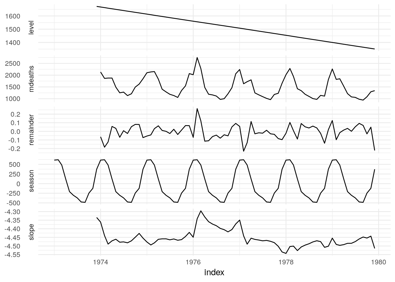
In many cases, a model can be used to extract features or components from data in a similar way to decomposition methods. We use the components verb to extract a tsibble of data features that have been extracted via modelling or decomposition.
State space models such as ETS are well suited to this functionality as the states often represent features of interest.
UKLungDeaths %>%
  model(ETS(mdeaths)) %>%
  components
## # A dable: 84 x 7 [1M]
## # Key: .model [1]
## # ETS(M,A,A) Decomposition: mdeaths = (lag(level, 1) + lag(slope, 1) +
## # lag(season, 12)) * (1 + remainder)
## .model index mdeaths level slope season remainder
## <chr> <mth> <dbl> <dbl> <dbl> <dbl> <dbl>
## 1 ETS(mdeaths) 1973 Jan NA NA NA 611. NA
## 2 ETS(mdeaths) 1973 Feb NA NA NA 620. NA
## 3 ETS(mdeaths) 1973 Mar NA NA NA 483. NA
## 4 ETS(mdeaths) 1973 Apr NA NA NA 122. NA
## 5 ETS(mdeaths) 1973 May NA NA NA -207. NA
## 6 ETS(mdeaths) 1973 Jun NA NA NA -304. NA
## 7 ETS(mdeaths) 1973 Jul NA NA NA -370. NA
## 8 ETS(mdeaths) 1973 Aug NA NA NA -476. NA
## 9 ETS(mdeaths) 1973 Sep NA NA NA -485. NA
## 10 ETS(mdeaths) 1973 Oct NA NA NA -246. NA
## # … with 74 more rows## Warning: Removed 11 rows containing missing values (geom_path).
It may also be worth storing how these components can be used to produce the response, which can be used for decomposition modelling.